Tag Archives: Genome Browser

October 2, 2014 · 10:51 am

Retooling Analysis Pipelines from Human to EBOV NGS Data for Rapid Alignment and Strain Identification

Screen Shot 2014-10-01 at 12.26.01 PM Can we use pipelines developed for human NGS analysis and quickly apply them for viral analysis? With ebolavirus being in the news, it seemed like a good time to try. Just as with a human sequencing project, it’s helpful if we have a good reference genome. The NCBI has four different ebola strain reference files located at their ftp:
Remote directory: /genomes/Viruses/* Accession: NC_002549.1 : 18,959 bp linear cRNA Accession: NC_014372.1 : 18,935 bp linear cRNA Accession: NC_004161.1 : 18,891 bp linear cRNA Accession: NC_014373.1 : 18,940 bp linear cRNA

Currently everything that’s happened in West Africa looks to match best with NC_002549.1, the Zaire strain. The Broad Institute began metagenomic sequencing from human serum this summer and the data can be accessed here (Accession: PRJNA257197). We can take some of these datasets and map them to NC_002549.1. The datasets are in .sra format, and must be extracted using fastq-dump.

Coverage map of SRA data from 2014 outbreak in Sierra Leone to the Zaire reference genome.

We can see that the data maps really well to this strain. All four of the reference genomes above were indexed with a new build of bwa(0.7.10-r876-dirty git clone https://github.com/lh3/bwa.git). Because EBOV genomes are so small, compared to humans, the only alignment algorithm which seemed suitable within bwa, was mem.
EBOV mokas$ ./bwa/bwa mem Zaire_ebolavirus_uid14703.fa SRR1553514.fastq > SRR1553514.sam [M::main_mem] read 99010 sequences (10000010 bp)... [M::mem_process_seqs] Processed 99010 reads in 8.988 CPU sec, 9.478 real sec [M::main_mem] read 99010 sequences (10000010 bp)... [M::mem_process_seqs] Processed 99010 reads in 8.964 CPU sec, 9.671 real sec
If we take the same SRA data and try to map it to some of the other strain references, e.g. the Reston Virginia strain from 1989, it can help give a rough idea of how closely related the 2014 incident is.

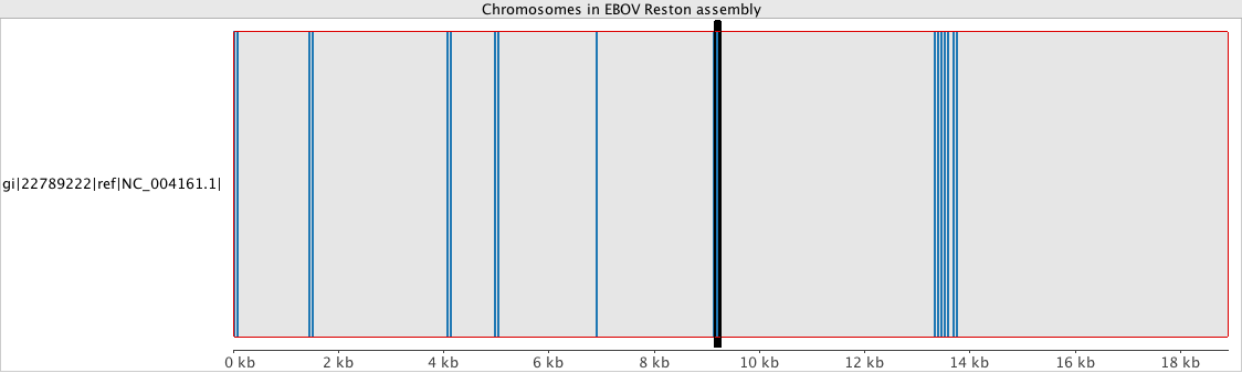
Very few regions from 2014 map to the Reston reference

It can be seen that apart from a few highly conserved regions where many reads align, the coverage map indicates that the data collected in West Africa and sequenced on the Illumina HiSeq2500 does not match to NC_004161.1. There were still approximately 500 variants with the Zaire reference on the 2014 samples, showing a good amount differences, considering the entire genome is only 18,000bp.

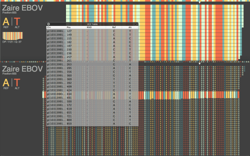
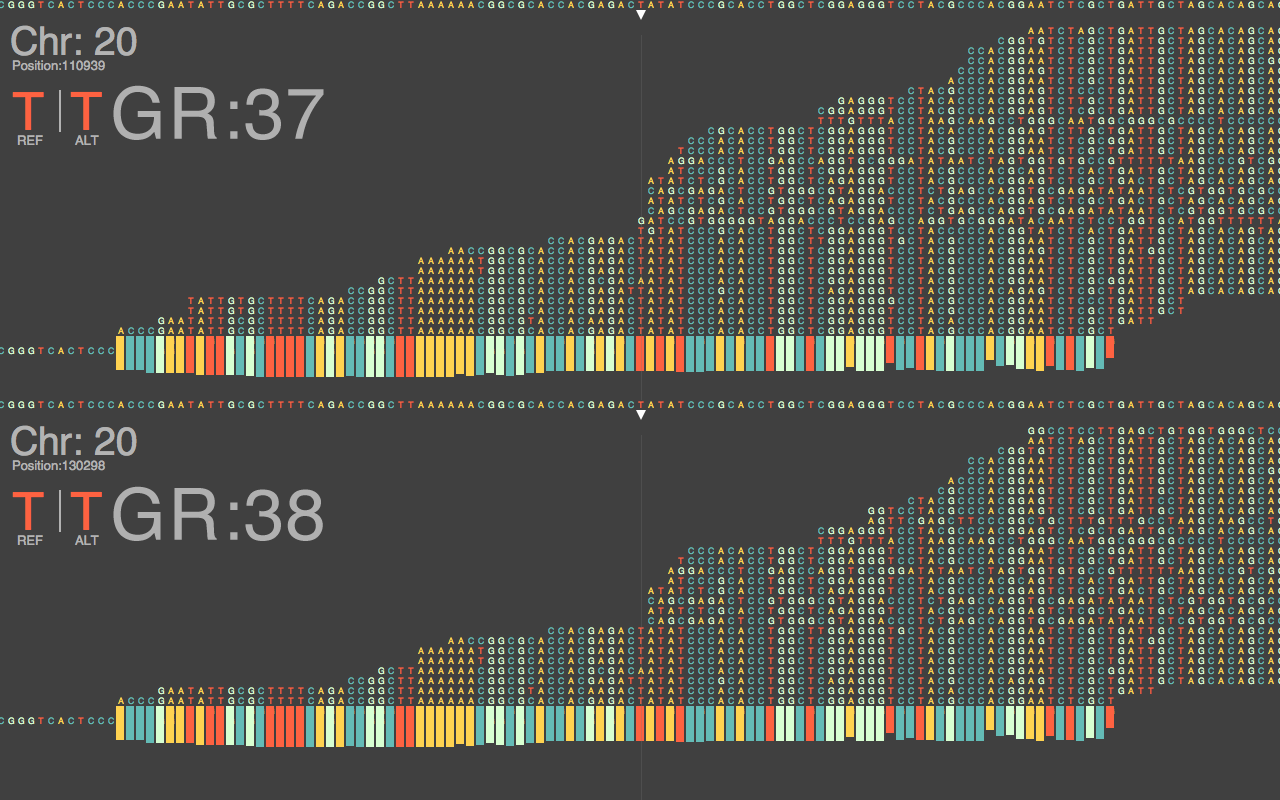
LucidAlign genome browser comparing the two strains

All of this is, of course, good news. We can take sequencing data of new EBOV strains and apply slightly modified pipelines to get meaningful results. And with the Ion PGM now being FDA approved means data can be generated in nearly 3 hours, with Federal approval.There have even been some publications which show that the protein VP24 can stop EBOV all together [DOI: 10.1086/520582] with the structures available for analysis as well. So, it looks like it’s all coming up humanity, our capabilities are there, and with proper resources this scary little bug can be a thing of history.

Hybrid Assemblies From Short and Long-Reads for INDEL Resolution, Finding The Missing Puzzle Piece

When it comes to genomics, contemporary bioinformatics follows the dogma of, assemble, detect, and annotate. This over-simplification however, washes over many key features, such as insertions and deletions, which may in fact be pathogenic[1].

Fig 1: A Low Complexity Region, featuring Homopolymers, leading to Ambiguous Mapping

High throughput, NGS short read data, and the algorithms developed to support them have overwhelmingly focused on detection of SNPs, while processing Structural Variants as an afterthought. This has largely been due to the combined limitations of chemistry and computation. Popular sequencers (I’m looking at you Illumina) produce strings with character lengths of several hundred bases. Matching millions of string-sets across highly-repetitive regions, where a single character or pattern of characters repeats over and over, is a nightmare from a algorithm design perspective.

Using Haplotype Calculations with Dindel, SeqAn, and Boost to Resolve INDELs

Fig 2: Using Haplotype Calculations with Dindel, SeqAn, and Boost C++ Libraries to Resolve INDELs

Because scientists and engineers are a lazy bunch with deep-rooted personality flaws, we’ve brushed the problem of sequence alignment in repetitive and low complexity regions under the rug. Sure, most aligners and callers will have some implementation for INDEL realignment, and detection (say Picard or Haplotype Caller in GATK), but if you’ve ever seen the results you know they don’t hold up well to scrutiny. Amongst this, the work of Kees Albers stands out, and anyone who has written a validated pipeline will attest to the results by Dindel’s four step process[2]:

$dindel --analysis getCIGARindels --bamFile sample.bam
        --outputFile sample.dindel_output --ref ref.fa

$python makeWindows.py 
        --inputVarFile sample.dindel_output.variants.txt
        --windowFilePrefix sample.realign_windows
        --numWindowsPerFile 1000

$while count < total.realign_windows:
       dindel --analysis indels --doDiploid 
              --bamFile sample.bam --ref ref.fa
              --varFile sample.realign_windows.2.txt
              --libFile sample.output.libraries.txt
              --outputFile sample.stage2_windows.2
       count +1

$mergeOutputDiploid.py 
        --inputFiles sample.dindel_stage2_out.txt
        --outputFile variantCalls.VCF --ref ref.fa

The process outlined above is quite compute intensive, and as can be seen in Figure 2, the number of possible haplotypes to resolve a single potential INDEL can range in the triple digits; each of which has to be aligned, and selected for by statistical relevance. Guillermo del Angel gives a great outline for those who use GATK (we find the results from Samtools more agreeable) to utilize Dindel, however even this has a fairly significant false positive rate[3].

Fig 3: GATK with Dindel Still has High FPR

An algorithm, regardless of how well designed, can’t overcome bad input data. And short reads are simply not good starting material for resolving structural variants. Luckily, several companies have taken on the challenge of developing long-read technologies, where the string lengths can reach tens of thousands of characters. We’ve been lucky enough to work with Pacific Biosciences, using data generated with their SMRT hardware and P5-C3 chemistry. Reads in suspected SV regions were extracted, the long reads were used to span the low-complexity/highly repetitive regions, and short reads reassembled using bayesian and HMM methods available in SeqAn and Boost.

Fig 4: Hybrid alignment in Lucid genome browser

At this point I should mention that while Boost is absolutely fabulous in-terms of providing great tools for C++ development, which is a great way to handle compute intensive tasks, it is without a doubt: pull-your-hair-out-frustraiting to build and use. Moreover, while our methods have significantly decreased the number of total SVs in our results, we haven’t had the chance to do a rigorous comparison for FPR; but I think a good way to do that would be similar to what Heng Li has shown recently[4].

Not a Big Deal, GRCh38: A Semi-Casual Comparison of the New Human Reference Genome

Over christmas the Genome Reference Consortium gave all of us doing in silico life-science a wonderful present, or maybe it was just a lump of coal. GRCh38, the newest human reference genome assembly, was released to cheers and jeers abound.

Fig.1: Chromosome 20 Assembly With BWA

Of course, most of us are excited to have up-to-date standards, especially with something like the human reference playing such a pivotal role in clinical adoption of genomics. However, some are lamenting the perhaps inevitable remapping of their NGS reads to this new reference. And it’s completely reasonable to have this worry. Will previous results from samples remain valid once assembled with this new reference, and how different will the sequence alignments be?

Fig.2: Ts/Tv Ratios between GRCh37 & 38

It will take months and years to thoroughly answer these questions, and notice the complete impact of this update on current NGS data. Consequentially, this does not keep us from starting to get preliminary ideas of what to expect in the coming years of working with this build. Figure 1 above, shows a nucelotide-level closeup of a BWA sequence alignment of the same dataset, generated on a HiSeq 2500, across the last major release of GRCh37 and the new GRCh38.

Internally we have been using chromosome 20 of human reference builds to benchmark tools and pipelines with datasets; it has a favorable size in terms of length, and not too many curveballs in terms of features. Figure 2 to the left, shows the Ts/Tv ratios between the two alignments of the same data across the two references to be quite similar at 0.3527 and 0.3445, respectively. Working with the slew of aligners, BWA has repeatedly shown itself to produce reliable results, while avoiding any overly-complex algorithms and trendy implementations. It’s a good workhorse.

Similarly, samtools was used to parse through our SAM/BAM files to produce VCFs with mpileup. Which, again, does not have the most bells and whistles, but is consistently reliable and good for comparing a single variable, in this case, the reference.

Fig.3: High-level Alignment Map Topology

Quantifiably, GRCh38 is very similar to the later GRCh37 releases, showing a change rate of 1 change every 159,558 bases on 37.69 and 1 change every 156,779 bases on 38 for our chromosome 20 dataset. Which, to use a technical term, looks pretty damn close. One of the major updates according to the GRC are changes to chromosome coordinates, which some back of the envelope math seems to give a Δ of +19,359 between GRCh37.69 and 38. In combination with one of the other major updates, sequence representation for centromeres, short-reads appear to be spread thinner to cover this difference, resulting in slightly lower depth of coverage versus 37.69. Figure 3 above, shows that overall the alignment map remains mostly similar, at least when BWA is used with standard Illumina reads; with somewhat negligible loss of DP.

Fig.4: Chr20 Annotation of Regional Structure

Fig.4: Chr20 Annotation of Regional Features

By far the largest noticeable change brought to preexisting datasets appears to be related to annotation. Figure 4 above, shows just how hopelessly incongruent GRCh38 is at the moment with current annotation resources, yielding the largest differences to the latest GRCh37 assembly for the same reads. But this was to be expected, annotation will very likely be the last to catch up to this new build, and will improve over months and years.

Fig.5: Pileup Difference

So, should your project start using GRCh38? The short answer is, not yet. The long answer, it depends on your project resources, pipeline flexibility, and the questions trying to be answered. It’s helpful to remap preexisting NGS data to this new reference, and newly generated datasets would benefit the most, as sequence alignment tends to be the most expensive process in the pipeline to redo. Just keep in mind that for useful results your entire analysis pipeline, which is often an amalgamation of various opensource, commercial, and internal components has to work together. For the time being, GRCh38 is a wrench in the gears for many people, but it has a very promising future.

3 Comments

Filed under Genome Browser, Genomics, LucidViewer

Tagged as Bioinformatics, C#, Genome Browser, Genomics, GRCh38, LucidAlign, reference genome assembly, Xamarin